Monte Carlo Estimation of Pi

Yesterday, I came across a neat way to approximate π using Monte Carlo simulation. I hadn’t seen this exercise before, but I think it is understandable and illustrative, so I decided to give it a try using both Excel and Python.

How it Works

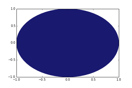
Imagine we have a unit circle inscribed within a 2×2 square.

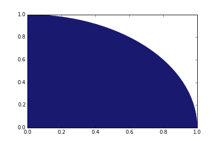
Now, let’s zoom into the top-right quadrant of this plot.

The area of this entire quadrant is equal to r² (since the base of the square equals the circle’s radius). The area in blue is a quarter-circle and is equal to (1/4)πr². Thus, if one were to plot points within this quadrant at random, we would expect that π/4 (approximately 78.54%) would lie within the blue region. Theoretically, then, to estimate π, one can generate a bunch of coordinate pairs with x and y values between 0 and 1. If the distance of a particular point from the origin is greater than 1 (greater than the radius of the circle), it is classified as outside of the circle. Otherwise, it is contained within the circle. With a large enough sample, the proportion of points within the circle should be close to π/4. We can then multiply this proportion by 4 to estimate π.

To get the distance of a point from the origin, we use the Pythagorean theorem:

Distance=sqrt(x² + y²).

Executing this using Excel

To carry out this process in Excel, I created two separate sets of 11,175 random numbers between 0 and 1 using the =RAND() function. I then calculated the distance for each pair. Next, I used an =IF() function to generate indicator variables corresponding to whether or not the calculated distance was greater than 1. Finally, I used =COUNTIF() to count those distances less than or equal to 1, divided this count by the total number of distances calculated (11,175), and multiplied this fraction by 4 to get an estimate of π.

Once all of this is in place, it is quick and easy to get estimates by pressing F9 to refresh the random numbers.

Here are 10 of the estimates I generated (accurate to 5 digits):

3.14917, 3.12447, 3.14309, 3.13879, 3.14452, 3.14130, 3.12197, 3.12841, 3.13128, 3.15347

For reference, the true value of π to 5 digits is 3.14159.

Here is a spreadsheet setup to carry out this simulation exercise.

Executing this using Python

I also replicated this process using Python. When replicating this process programatically, it is much easier to increase the scale (i.e., number of distance estimates).

Here is my Python code:

#single point estimate
import random
from math import *
from __future__ import division

n=100000 #number of random number pairs

my_randoms = [] #create empty list to store distance calculations

for _ in range(0,n):
    my_randoms.append(sqrt((random.random()**2) + (random.random()**2))) #distance calculation
    
pi_estimate=(sum(x<=1 for x in my_randoms)/n)*4

print pi_estimate

Using 100,000 random number pairs, here are 10 estimates that I got:
3.12924, 3.16036, 3.14132, 3.14204, 3.13932, 3.13904, 3.1464, 3.14028, 3.14208, 3.13856

Simulating this process programatically also allowed me to go one step further. Again, I used the random number pairs to generate an estimate of π (this time “only” 10,000 pairs to spare my computer from the extra calculations). However, using a nested for-loop, I repeated this process 10,000 times! One can then take the average of the 10,000 π estimates to get an even better approximation of π. Additionally, one can test the validity of the Central Limit Theorem to see if the 10,000 estimates are normally distributed.

Here’s my Python code to do just this:

#average of 10,000 estimates; takes some time to run
import random
from math import *
from __future__ import division
import matplotlib.pyplot as plt

n1= 10000 #number of pi estimates 
n2= 10000 #number of random number pairs to use in pi estimate

pi_list=[] #create empty list to store pi estimates

for _ in range(0,n1): #n1 iterations
 my_randoms=[] #create empty list to store distance calculations
 for _ in range(0,n2):
 my_randoms.append(sqrt((random.random()**2) + (random.random()**2))) #distance calculation
 pi_list.append((sum(x<=1 for x in my_randoms)/n2)*4)

print sum(pi_list) / float(len(pi_list)) #average pi estimate

plt.hist(pi_list) #histogram of pi estimates

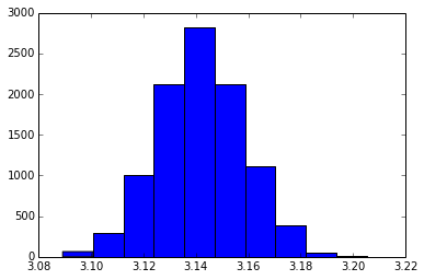
Using this program, my distribution of π estimates looked like this:

Without any hesitation, I would say that the estimates follow a normal distribution.

After only one execution of this program, I received a π approximation (based on the average of 10,000 estimates) of 3.14168, which is just .00009 off from the true value of π.